The FILTER function in Google Sheets allows you to filter data and return rows that meet specific criteria. Below is how to use the FILTER function in Google Sheets .
- Google Sheets - Google Sheets
- Google Sheets for iOS
- Google Sheets for Android
Overview of the Filter function formula in Google Sheets
By using this Google Sheets function, you can get multiple matches. Because the data is filtered using the function, the results will be updated automatically.

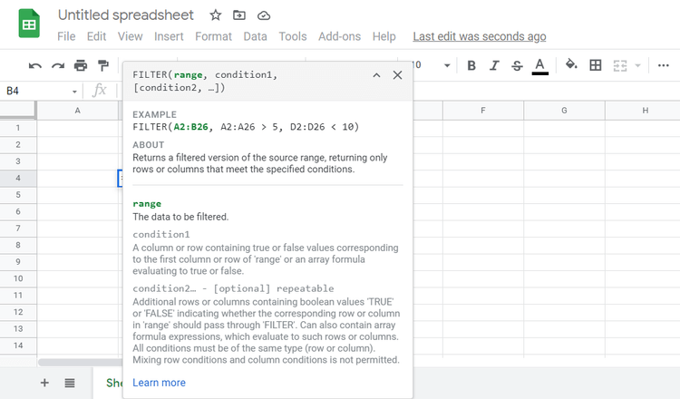
The Google Sheets Filter function formula includes: Range - Range, Condition 1 - Condition 1, and [Condition 2…]. The first two factors are mandatory, while the second and subsequent conditions are optional. Google Sheets does not limit the number of conditions in the Filter function.
=filter(range, condition 1, [condition 2]…)
- Range : Range to filter data in an array. It can contain any number of rows or columns.
- Test condition 1 : Condition that determines whether a value is true or false in a column or row.
- [Condition 2…] : It refers to additional rows or columns containing logical values: TRUE or FALSE according to the criteria in the filter.
Example of using the Filter function in Google Sheets
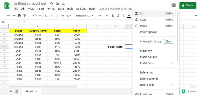
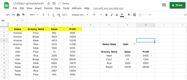
You can find information about sales and profits of each item in different states in the US when using the Filter function in Google Sheets. When a column containing the state name is condition 1, you can create a drop-down list for it.
Create drop-down lists for test conditions
1. Right-click a cell to open the drop-down menu.

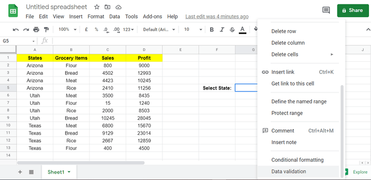
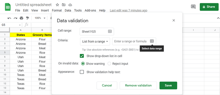
2. Scroll down and go to the Data validation section .

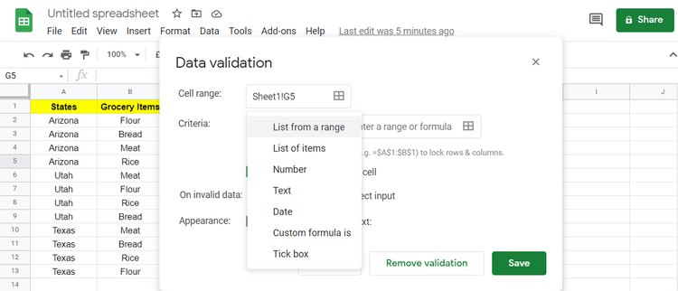
3. In the data validation section, set the criteria to List from a range.

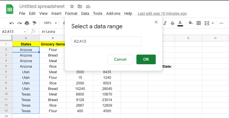
4. Click the squares in the criteria section to select a range or formula.

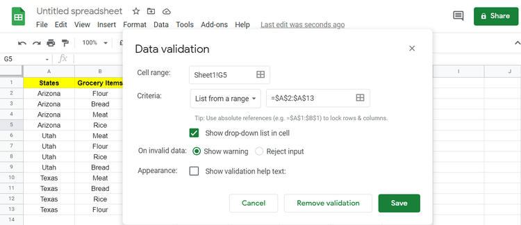
5. In this case, the States column will be the range. You need to select items from cells A2 to A13 here.

6. Save the Data Validation settings by clicking Save .

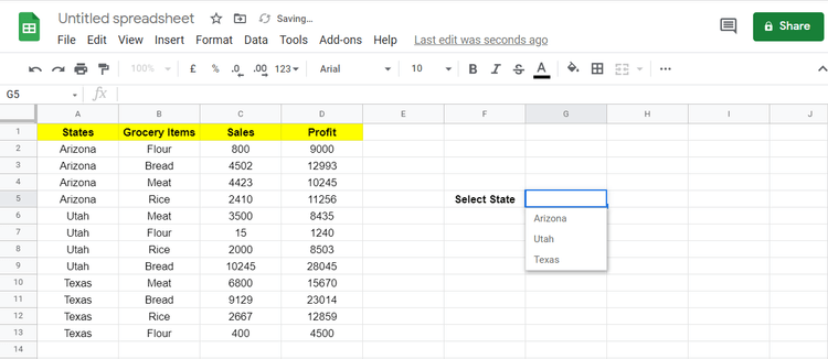
This action will create a drop-down menu containing items specific to the selected range.

Now that you have created the drop-down menu, start filtering Grocery Items, Sales and Profit by States using the Filter function on Google Sheets.
Implement the Filter function
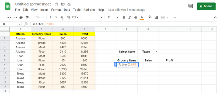
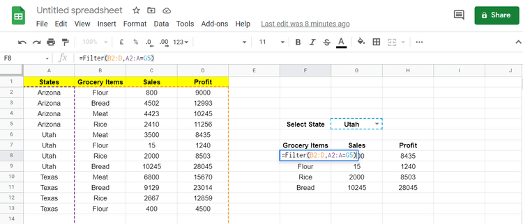
Here the range is data in 3 columns: Sales, Grocery items and Profit. Now select cells B2 to D13 in the first argument of the Filter function.

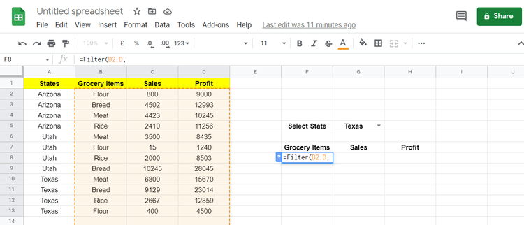
Suppose you want to add more data to the column selected as a range. Remember the second value in the open range. You can do this by deleting the number of cells, here it is 13.

As soon as a new value is added, the Filter function will calculate these values without requiring you to filter them again.
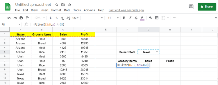
The condition value in this example is the States column. Select the States column and set the condition that that column = with the data in cell G5.

In this example, Range Area B2:D has the same height as condition area A2:A.
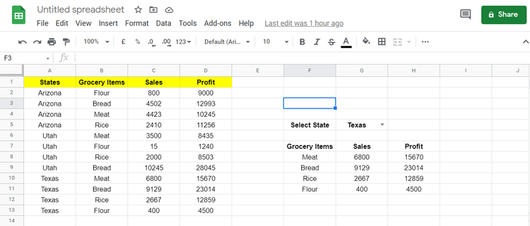
After pressing Enter to deploy the formula, it will filter the data in the Grocery items, Sales, Profits columns according to the given conditions.

Also, note that the Google Sheets Filter function only includes valid values. If the value checks true, its value in the array is considered, otherwise the function ignores it and moves on to the next step.
In this example, when you select Utah from the drop-down list, you'll see the related data in the filter area.

Filter data by checking multiple conditions
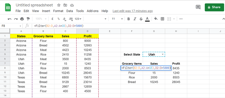
Now we'll update the Google Sheets Filter function to include values greater than 5000 as the second condition. To filter data that meets both conditions, you need to add a new condition to the filter formula.
1. Go to cell F8 where you added the formula earlier.

2. Select the Profit column as the range for the second condition, the new formula is as follows:
=Filter(B2:D,A2:A=G5,D2:D>5000)

3. Press Enter to execute the formula.

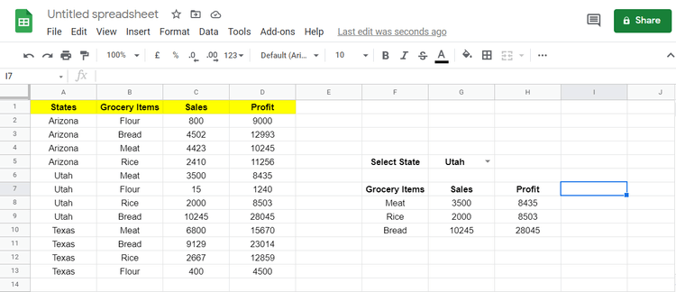
The profit from selling flour in Utah is 1240, which does not meet the second condition, so the Filter function of Google Sheets ignored it. Similarly, you can filter this data by trying more conditions.
Above is how to use the Filter function in Google Sheets . Hope the article is useful to you.

