How to Copy Partition to Another Drive in Windows 11/10/8/7
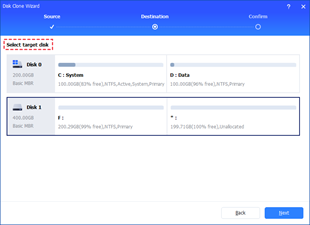
In Windows 11, 10, 8, and 7, you can quickly copy a partition to a different drive using the flexible disk cloning tool AOMEI Partition Assistant.
If you have been using Google Sheets for some time now, you might already be familiar with the different functions for counting cells. Depending on what type of cells you want to count—blank or non-blank, colored or bold—there are various functions that can help you. But what happens when your spreadsheet contains unique values? This is where the COUNTUNIQUE formula comes in.

In this article, we’ll discuss how to count unique values in Google Sheets using the COUNTUNIQUE formula. We’ll also talk about counting unique values in a single column.
How to Count Unique Values in Google Sheets
Knowing how to count cells in Google Sheets can be useful for many reasons, especially if you’re working with a large dataset. If you only have a small amount of data, you would be able to count the number of specific cells manually. Google Sheets offers various functions for counting different types of cells in a specific data range, including blank cells, text cells, colored cells, bold cells, and more. These are called COUNT functions.
In some cases, you might be required to know the number of unique values in your spreadsheet. For example, you might need to know how many times a certain name or product appears in your spreadsheet. For this, we will be using the COUNTUNIQUE function. It’s used to count the number of unique values in a range or some kind of specified list. To be more precise, you can use the COUNTUNIQUE formula for dates, numbers, names, products, cell references, or random data.
You can also use the COUNTUNIQUE formula to see if there are any duplicates of the unique value. This helps you find errors in your spreadsheet and makes it generally easier to keep track of all your data.
To count unique values in Google Sheets, follow the steps below.


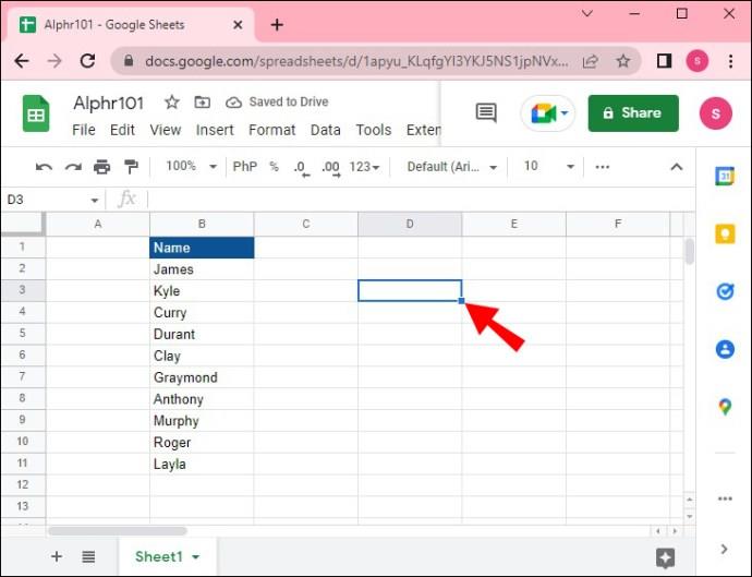
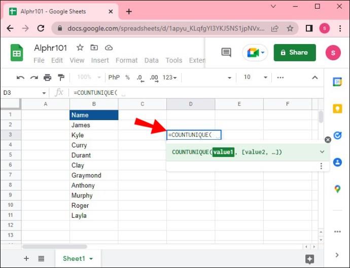

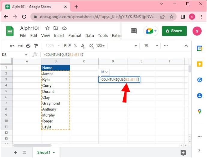
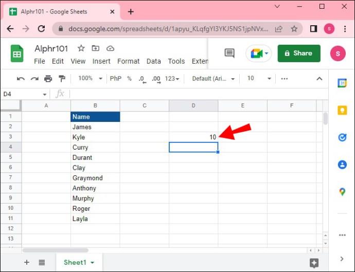
The number of the unique values in your spreadsheet will appear in the empty cell where you wrote the formula. For example, if you see the number “7” in the cell, it means there are seven instances of unique values in the spreadsheet.
The COUNTUNIQUE formula is used to count the number of unique values within a specific range. But what if you want to find the exact unique values? In this case, we will be using the UNIQUE function, without the COUNT.
For example, say you wrote the names of all your students in one spreadsheet, and you want to see how many students have the same name. Similarly, if you have compiled a list of various products, the UNIQUE function can help you identify which product names are duplicates.
Here’s how you can use the UNIQUE function to display the unique values in your Google Sheets spreadsheet.


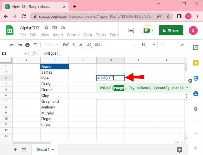
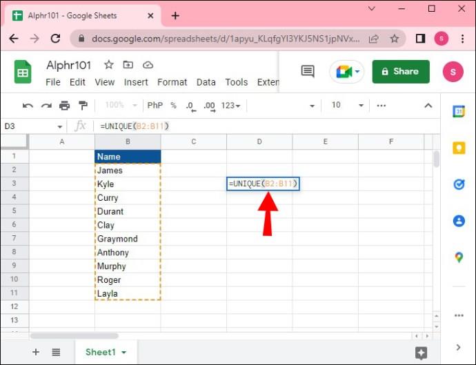
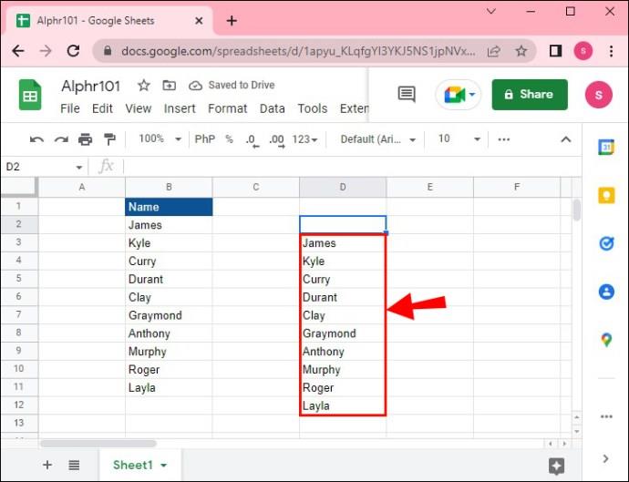
All the unique values will be displayed in the form of a list. You can use this formula to see if there are any duplicates in the sheet and then remove them if that’s your goal.
Google Sheets Count Unique Values in Column
Using the COUNTUNIQUE formula to count unique values in a single column is even easier than doing so for a bigger range. Here’s how it’s done.


That’s all there is to it. The number of unique values will appear in the cell where you entered the formula.
Keep Track of All the Unique Values in Google Sheets
Although using functions to count values in Google Sheets may seem confusing at first, you’ll get the hang of it in no time. The COUNTUNIQUE formula is very useful for counting unique values in a selected data range, and it can even help you find duplicates.
Have you ever used the COUNTUNIQUE function to count unique values in Google Sheets? Did you use the instructions from this guide, or another method? Tell us about your experience with Google Sheets functions in the comments section below.
In Windows 11, 10, 8, and 7, you can quickly copy a partition to a different drive using the flexible disk cloning tool AOMEI Partition Assistant.
Driver Booster 12 Free is an effective tool that will keep your computers drivers up to date, which will make the system run faster and more reliably. This driver updater from IObit keeps your PC running at its best by checking for lost, out-of-date, or broken drivers immediately.
In an era where digital efficiency is paramount, Advanced SystemCare 17 Free emerges as a beacon for those seeking to enhance their PC's performance.
Summary of Movies & TV application shortcuts on Windows 10, Summary of Movies & TV application shortcuts on Windows 10 to bring you a great experience. Maybe
How to fix Messages Failed to Load error on Discord for Windows, Discord isn't fun if you can't read what other people write. Here's how to fix Messages error
How to display the This PC icon on the Windows 11 desktop, During the process of using Windows 11, many users need to access This PC (management).
How to find information in the Windows Registry quickly, Do you find it difficult to find information in the Windows Registry? So below are quick ways to find the registry
How to limit the number of failed login attempts on Windows 10. Limiting the number of failed password login attempts on Windows 10 helps increase computer security. Here's how
How to create fake error messages in Windows, Windows can come up with some pretty creative error messages but why don't you try creating your own content for them to make fun of?
Ways to open Windows Tools in Windows 11, Windows Administrative Tools or Windows Tools are still useful on Windows 11. Here's how to find Windows Tools in Windows 11.
How to fix Windows Quick Assist not working error, Windows Quick Assist helps you connect to a remote PC easily. However, sometimes it also generates errors. But,
How to pin Word, Excel and PowerPoint files to the corresponding app icon on the Windows 11 taskbar, How to pin Office files to the taskbar icon on Windows 11? Invite
How to fix the error of not being able to install software on Windows, Why can't you install apps or software on Windows 10/11? Here's everything you need to know about how to fix it
Instructions for deleting or changing the PIN code on Windows 11, In Windows 11, the PIN code is a very useful and convenient security tool for users. However some people
How to fix There Are Currently No Power Options Available error in Windows 10, Can't select power mode in Windows 10, what should I do? Here's how to fix the error
The simplest way to fix Photos app errors on Windows 10, what should I do if Microsoft Photos doesn't work? Don't worry about ways to fix Photos app errors on Windows
Instructions for installing shortcuts to switch input languages on Windows 11. During the process of using Windows, users will often have to switch between methods.
How to check power status is supported on Windows 11, Windows 11 can handle many different power states. Here's how to check the power status
How to switch from 2.4GHz to 5GHz in Windows 10, If you want to find a quick and simple way to speed up the Internet, changing the WiFi band from 2.4GHz to 5GHz may help.
How to fix Not Enough Memory to Run Microsoft Excel error on Windows, Are you having an error of not enough memory to run Microsoft Excel? So, how to fix Not Enough Memory error


