The Best Diets for Heart Health

In addition to regular exercise and not smoking, diet is one of the best ways to protect your heart. Here are the best diets for heart health.
The Vlookup function is a function that searches for values to return other values in an existing worksheet. The Vlookup function is one of the most used functions in Excel , applying to many practical tasks such as calculating electricity charges based on electricity numbers, giving academic results based on average score, taking data on place of birth, gender Employee calculation based on employee name or code ...
Although the applicability is very high, many people still do not understand the nature of this function like? Syntax like? How to use this function? So please refer to the following article of Download.com.vn to better understand:
Syntax:
= VLOOKUP (lookup_value, table_array, col_index_num, [range_lookup])
Quick explanation: VLOOKUP (The value you want to look up, the range in which you want to find the value, the number of columns in the range containing the return value, Exact or Relative return results - expressed as 0 / FALSE or 1 / TRUE)
Explain each value:
Relative searching with the Vlookup function is a way of finding relative data based on the difference between the first column data of the search area. To find relative results that return true results, your original data table (which is your Table_array table ) is required to sort in ascending order.
Example 1: Please classify students in the list below, based on the table of rules of grading by:
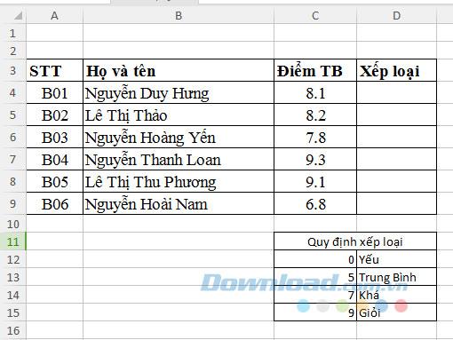
To classify academic performance for a student list, use the formula:
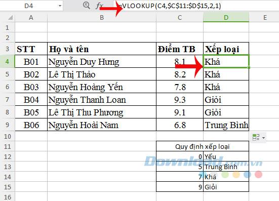
=VLOOKUP(C4,$C$11:$D$15,2,1)
Then press Enter , then scroll down to the remaining cells you will get the results as shown below:
Example 2: Based on the employee code table below, fill in their Qualifications and Hometown .
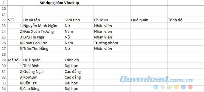
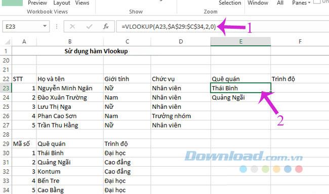
To fill in the Employee Information field of cell E23 use the following formula:
=VLOOKUP(A23,$A$29:$C$34,2,0)
And here is the result:
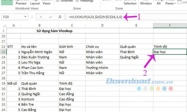
Also fill in the Level for F23, use the following formula:
=VLOOKUP(A23,$A$29:$C$34,3,0)
And this will be the result that will be obtained:
In addition to the simple usage as above, you can customize to have a more flexible Vlookup function, especially in cases where the search data table is too wide and the column counting becomes ... tiring.
The MATCH function looks for a specified value in a range of cells, then returns the relative position of that value in this range. For example, if the range A1: A3 contains values 5, 10 and 15, the formula = MATCH (10, A1: A3,0) will return the number 2, because 10 is the second value in the range A1: A3. The syntax of the Match function is as follows:
= MATCH (lookup value, lookup array, [match type])
So, where does the Match function apply to Vlookup? Please tell you it is in the value Col_index_num - the column to get data. Putting it into a specific example will make it easier for you to imagine.
Example: Given the following data table:

Need to filter the data by month for each employee in the main table (the month column in the main table may vary). Specifically, the spreadsheet will look like this:
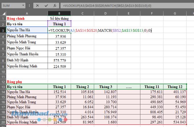
The formula used in the lesson:
= VLOOKUP (A3; $ A $ 14: $ G $ 20; MATCH ($ B $ 2; $ A $ 13: $ G $ 13; 0) ; 0)
The Match function will help you count the number of columns to be retrieved in the lookup data table (side table) of the Vlookup function. So, just change the Month data in cell B2 , you will have the exact data for each corresponding month. In the following example, I change the month column data in the Main Table and the result is:
Also one of the most used functions, Left / Right and Mid can combine with Vlookup and make miracles in search.
Example: For the following table, fill in the blank data based on the sub tables below:
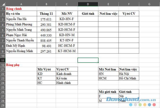
The input data to fill in the data is described as follows: The first 2 characters of the Employee descriptor code for the job position, the middle character in the gender description, the characters at the end of the description for the multiplier tablets work. Based on that, we will fill in the formula for calculating each column as follows:
| CV position | = VLOOKUP ( LEFT (C3; 2) ; $ B $ 22: $ C $ 24; 2; 0) |
| Workplace | = VLOOKUP ( RIGHT (C3; LEN (C3) -5) ; $ E $ 22: $ F $ 23; 2; 0) |
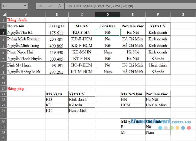
| Sex | = VLOOKUP ( MID (C3; 4; 1) ; $ E $ 27: $ F $ 28; 2; 0) |
And this is the result:
The #NA error stands for Not Available Error which means the corresponding value cannot be found. It is possible that in this case you have used absolute search and the data you are looking for is not in the range containing the lookup value ( Table_array ).
There are many reasons for this: it is possible that the lookup value ( Lookup_value ) in the main table and sub-table (in the above example) is different with only one space (space), the data cannot be found. or you get the wrong part of the Table_array area so that the data to be searched ( Lookup_value ) is not in the first column of the Table_array ...
So, depending on the specific case, you need to fix the #NA error in Vlookup function properly, just remember only one thing: the data to be searched should be absolutely right with the first column of the table containing the lookup value. If absolute searching is used (Range_lookup = 0) .
So you already know how to use the Vlookup function. In the process of using Excel you can also use the Index function to return values in an array or the Max and Min functions for the largest and smallest values.
When you master the syntax, how to use functions in Excel, you will learn Excel effectively, much faster. In addition, there are many other useful functions, Download.com.vn will introduce to you in the following articles.
I wish you successful implementation!
In addition to regular exercise and not smoking, diet is one of the best ways to protect your heart. Here are the best diets for heart health.
Diet is important to our health. Yet most of our meals are lacking in these six important nutrients.
At first glance, AirPods look just like any other true wireless earbuds. But that all changed when a few little-known features were discovered.
In this article, we will guide you how to regain access to your hard drive when it fails. Let's follow along!
Dental floss is a common tool for cleaning teeth, however, not everyone knows how to use it properly. Below are instructions on how to use dental floss to clean teeth effectively.
Building muscle takes time and the right training, but its something anyone can do. Heres how to build muscle, according to experts.
The third trimester is often the most difficult time to sleep during pregnancy. Here are some ways to treat insomnia in the third trimester.
There are many ways to lose weight without changing anything in your diet. Here are some scientifically proven automatic weight loss or calorie-burning methods that anyone can use.
Apple has introduced iOS 26 – a major update with a brand new frosted glass design, smarter experiences, and improvements to familiar apps.
Yoga can provide many health benefits, including better sleep. Because yoga can be relaxing and restorative, its a great way to beat insomnia after a busy day.
The flower of the other shore is a unique flower, carrying many unique meanings. So what is the flower of the other shore, is the flower of the other shore real, what is the meaning and legend of the flower of the other shore?
Craving for snacks but afraid of gaining weight? Dont worry, lets explore together many types of weight loss snacks that are high in fiber, low in calories without making you try to starve yourself.
Prioritizing a consistent sleep schedule and evening routine can help improve the quality of your sleep. Heres what you need to know to stop tossing and turning at night.
Adding a printer to Windows 10 is simple, although the process for wired devices will be different than for wireless devices.
You want to have a beautiful, shiny, healthy nail quickly. The simple tips for beautiful nails below will be useful for you.


