Guide to participating in Dynamax & Max battles in Pokemon Go

The exciting new Dynamax feature is here in Pokémon GO. Here's what you need to know about how to Dynamax and Max in Pokémon Go.
The COS function in Excel is a trigonometric function in Excel , which calculates the cosine of a given angle quickly and accurately as when you use a calculator. You can use the COS function in Excel to calculate a single calculation, or combine it with many other calculations to get the result for the calculation. Below are instructions for using the COS function in Excel.
How to use the COS function in Excel
The syntax of the COS function is =COS(number) where number is the angle in radians you want to find. If you want the argument in degrees, you need to multiply that number by PI()/180 or use the RADIANS function to convert it to radians. So you have 2 formulas to apply: =COS(RADIANS(number)) and =COS(number*PI()/180) to convert to radians before calculating cos.
Step 1:
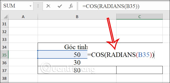
With the example table below, the user first needs to convert the angle to radians.

We combine the formula and enter it into any cell =COS(RADIANS(B35)) and press Enter.
Step 2:
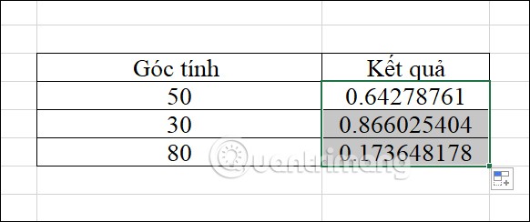
Immediately you have the result of the COS function in Excel as shown below. We just need to drag the result of this cell down to other cells.
Instructions for using the ACOS function in Excel
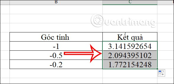
With the ACOS function in Excel, the user has the function syntax =ACOS(number) . In which number must be a number from -1 to 1. If the number to be calculated is not in this range, the ACOS function will return the error value #NUM!.
Step 1:
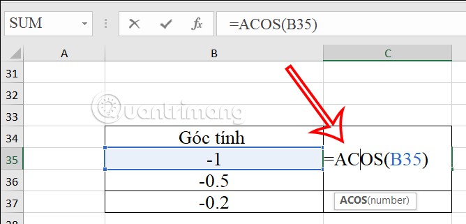
In the cell displaying the result, we enter the function =ACOS(B35) and press Enter to execute the function.
Step 2:
Then the user also sees the result for the ACOS function. You just need to drag the first result cell down to show the results for the remaining cells that need to be calculated.
The exciting new Dynamax feature is here in Pokémon GO. Here's what you need to know about how to Dynamax and Max in Pokémon Go.
Weibo social network also has the same setting options as other social networking applications such as changing Weibo account password or changing account name to a new name you like.
Batch files are a way for computer users to get work done. They can automate everyday tasks, shorten the time it takes to do something, and turn a complex process into something anyone can operate.
With the instructions in the article you can download and install Minecraft for free on iPhone/iPad
There are many different ways to change the default PDF reader on Windows 10, helping you get the PDF reader on your computer as you like through PDF reading software or even reading PDF files using a browser.
The Shortcuts app on iPhone has a shortcut to convert videos to GIFs with very simple operations.
Numerology reveals exactly what's in your name. From destiny to soul path, here's how to calculate your numerology chart based on your name.
WhatsApp has been updated with a new feature to select video callers in groups, no need to make a call with all members in the group. Here is a guide to select video callers in WhatsApp groups.
Meta AI has been updated on Messenger for you to experience this chatbot, interact with the chatbot for any issue you care about.
If you have a personal photo that you want to cover some information or even a certain image, you can insert stickers into the photo on iPhone.
For some reason, you no longer want to use your current Google account, and want to completely delete it. So how can you permanently delete your Google account?
You can now chat with the official ChatGPT on WhatsApp without resorting to third-party chatbots.
On Windows 11 you can now use the Copilot app to find, open, and ask questions about files stored on your computer.
iPhone 15 and later after upgrading to iOS 18 are equipped with new Apple Intelligence technology, capable of removing objects in photos via the Clean Up tool.
Not only does ChatGPT feature AI photo generation using your description, you can now create Snoopy style photos very simply.


